In a world where creativity is becoming more and more reliant on a solid understanding of mathematics, this course acknowledges the necessity for analytical proficiency. In addition to traditional pre-university mathematics topics (such as functions, trigonometry, and calculus), this course also covers topics that lend themselves to investigation, conjecture, and proof, such as the study of sequences and series at both the SL and HL levels and proof by induction at the HL level. The course permits the use of technology because proficiency with the required handheld and mathematical software is crucial regardless of the course you choose. However, the capacity to create, convey, and defend sound mathematical ideas is emphasized heavily in Mathematics: Analysis and Approaches.
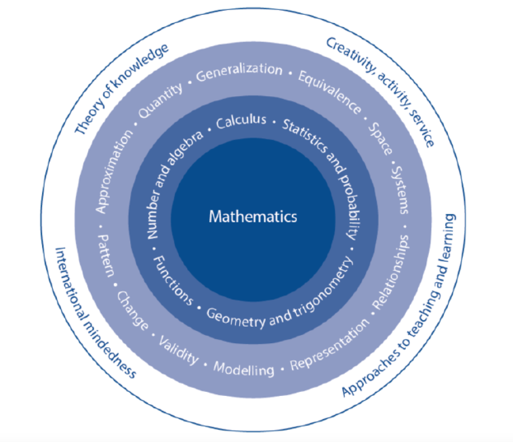
What is IB Math : Analysis and Approaches ?
In a world where creativity is becoming more and more reliant on a solid understanding of mathematics, this course acknowledges the necessity for analytical proficiency. In addition to traditional pre-university mathematics topics (such as functions, trigonometry, and calculus), this course also covers topics that lend themselves to investigation, conjecture, and proof, such as the study of sequences and series at both the SL and HL levels and proof by induction at the HL level. The course permits the use of technology because proficiency with the required handheld and mathematical software is crucial regardless of the course you choose. However, the capacity to create, convey, and defend sound mathematical ideas is emphasized heavily in Mathematics: Analysis and Approaches.
Students should appreciate seeing how mathematics is applied in real-world situations and to resolve real-world issues if they pick Mathematics: applications and interpretation at the SL or HL level. Students with a strong background in algebra and expertise with problem-solving in the real world will be prepared to study Mathematics: Applications and Interpretation at the higher level. These kids will enjoy and feel satisfied when they investigate complex issues, and they will feel at ease using technology to do so.
From the Following tables you can easily see the syllabus structure with recommended hours and assesment structure.
|
Syllabus component |
Recommended teaching hours |
|
19 21 25 27 28 |
|
Development of investigational, problem-solving and modelling skills and the exploration of an area of mathematics |
30 |
|
Total teaching hours |
150 |
|
Type of assessment |
Format of assessment |
Time (hours) |
Weighting of final grade (%) |
| External | |||
| Paper 1 |
No technology allowed. Section A: compulsory short-response questions based on the syllabus. Section B: compulsory extended-response questions based on the syllabus. |
1.5 | 40 |
| Paper 2 |
Technology allowed. Section A: compulsory short-response questions based on the syllabus. Section B: compulsory extended-response questions based on the syllabus. |
1.5 | 40 |
| Internal | |||
| Exploration | 15 | 20 |
Also from the following list you can see the detailed syllabus of IB SL Math AA.
SL-AA
- Topic 1 – Number and Algebra
1.1. Number Skills 1.1.1. Operations with numbers in the form a×10k where 1≤a<10 and k is an integer.
1.2. Sequences and Series 1.2.1. Arithmetic sequences and series.Use of the formulae for the nth term and the sum of the first n terms of the sequence.Use of sigma notation for sums of arithmetic sequences.
1.2.1.1. Applications (Examples incluede simple interest over a number of years.)
1.2.1.2. Analysis,interpretation and prediction where a model is not perfectly arithmetic in real life.
1.3. Geometric sequences and series.Use of the formulae for the nth term and the sum of the first n terms of the sequence 1.3.1. Use of sigma notation for the sums of geometric sequences.
1.3.2. Applications (Examples include the spread of disease,salary increase and decrease and population growth.)
1.4. Financial applications of geometric sequences and series.Compound Interest.Annual Depreciation
1.5. Laws of exponents with integer exponents. 1.5.1. Introduction to logarithms with base 10 and e.Numerical evaluation of logarithms using technology.
1.6. Simple deductive proof, numerical and algebraic; how to lay out a left-hand side to right-hand side (LHS to RHS) proof.The symbols and notation for equality and identity.
1.7. Laws of exponents with rational exponents.
1.7.1. Laws of logarithms.logaxy=logax+logay logax/y=logax−logay logaxm=mlogax for a, x, y>0
1.7.2. Change of base of a logarithm.logax=logbx/logba, for a, b, x>0
1.7.3. Solving exponential equations, including using logarithms.
1.8. Sum of infinite convergent geometric sequences.
1.9. The binomial theorem:expansion of (a+b)n,n∈ℕ. 1.9.1. Use of Pascal’s triangle and nCr.
2. Topic 2 – Functions
2.1. Different forms of the equation of a straight line.Gradient; intercepts.Lines with gradients m1 and m2.Parallel lines m1=m2.Perpendicular lines m1×m2=-1.
2.2. Concept of a function, domain, range and graph.Function notation, for example f(x),v(t),C(n).The concept of a function as a mathematical model. 2.2.1. Informal concept that an inverse function reverses or undoes the effect of a function.Inverse function as a reflection in the line y=x, and the notation f^-1(x).
2.3. The graph of a function; its equation y=f(x). 2.3.1. Creating a sketch from information given or a context, including transferring a graph from screen to paper.Using technology to graph functions including their sums and differences.
2.4. Determine key features of graphs 2.4.1. Finding the point of intersection of two curves or lines using technology.
2.5. Composite functions. 2.5.1. Identity function. Finding the inverse function f-1(x).
2.6. The quadratic function f(x)=ax2+bx+c: its graph, y -intercept (0,c). Axis of symmetry.The form f(x)=a(x−p)(x−q), x- intercepts (p,0) and (q,0).The form f(x)=a(x−h)2+k, vertex (h,k).
2.7. Solution of quadratic equations and inequalities.The quadratic formula. 2.7.1. The discriminant Δ=b2−4ac and the nature of the roots, that is, two distinct real roots, two equal real roots, no real roots.
2.8. The reciprocal function f(x)=1/x,x≠0: its graph and self-inverse nature. 2.8.1. Rational functions of the form f(x)=(ax+b)/(cx+d) and their graphs.Equations of vertical and horizontal asymptotes.
2.9. Exponential functions and their graphs:f(x)=ax, a>0, f(x)=ex.Logarithmic functions and their graphs:f(x)=logax, x>0, f(x)=lnx, x>0.
2.10. Solving equations, both graphically and analytically.
2.10.1. Use of technology to solve a variety of equations, including those where there is no appropriate analytic approach.
2.10.2. Applications of graphing skills and solving equations that relate to real-life situations.
2.11. Transformations of graphs.Translations: y=f(x)+b;y=f(x−a).Reflections (in both axes): y=−f(x);y=f(−x).Vertical stretch with scale factor p: y=pf(x).Horizontal stretch with scale factor 1/q: y=f(qx). 2.11.1. Composite transformations.
3. Topic 3 – Geometry and Trigonometry
3.1. 3D Geometry
3.1.1. The distance between two points in three-dimensional space, and their midpoint.
3.1.2. Volume and surface area of three-dimensional solids including right-pyramid, right cone, sphere, hemisphere and combinations of these solids.
3.1.3. The size of an angle between two intersecting lines or between a line and a plane.Trigonometry
3.2. Use of sine, cosine and tangent ratios to find the sides and angles of right-angled triangles. 3.2.1. The sine rule: a/sinA=b/sinB=c/sinC
▪ The cosine rule: c^2=a^2+b^2-2abcosC
▪ cosC=a^2+b^2-c^2/2ab
▪ Area of a triangle as 1/2absinC.
3.3. Applications of right and non-right angled trigonometry, including Pythagoras’ theorem.Angles of elevation and depression.
3.3.1. Construction of labelled diagrams from written statements.
3.4. The circle: length of an arc; area of a sector.
3.5. Definition of cosθ, sinθ in terms of the unit circle.
3.5.1. Definition of tanθ as sinθ/cosθ.
3.5.2. Exact values of trigonometric ratios of 0, π/6, π/4, π/3, π/2and their multiples.
3.5.3. Extension of the sine rule to the ambiguous case.
3.6. The Pythagorean identity cos2θ+sin2θ=1.Double angle identities for sine and cosine. 3.6.1. The relationship between trigonometric ratios.
3.7. The circular functions sinx, cosx, and tanx; amplitude, their periodic nature, and their graphs.Composite functions of the form f(x)=asin(b(x+c))+d.
3.7.1. Transformations.
3.7.2. Real-life contexts.
3.8. Solving trigonometric equations in a finite interval, both graphically and analytically. 3.8.1. Equations leading to quadratic equations in sinx,cosx or tanx.
4. Topic 4 – Statistics and Probability
4.1. Descriptive Statistics
4.1.1. Concepts of population, sample, random sample, discrete and continuous data.
4.1.2. Reliability of data sources and bias in sampling.
4.1.3. Interpretation of outliers.
4.1.4. Sampling techniques and their effectiveness.
4.2. Presentation of data (discrete and continuous): frequency distributions (tables).
4.2.1. Histograms.Cumulative frequency; cumulative frequency graphs; use to find median, quartiles, percentiles, range and interquartile range (IQR).
4.2.2. Production and understanding of box and whisker diagrams.
4.3. Measures of central tendency (mean, median and mode).Estimation of mean from grouped data.
4.3.1. Modal class.
4.3.2. Measures of dispersion (interquartile range, standard deviation and variance).
4.3.3. Effect of constant changes on the original data.
4.3.4. Quartiles of discrete data.
4.4. Linear correlation of bivariate data.
4.4.1. Scatter diagrams; lines of best fit, by eye, passing through the mean point.
4.4.2. Equation of the regression line of y on x.
4.5. Concepts of trial, outcome, equally likely outcomes, relative frequency, sample space (U) and event.
4.5.1. Expected number of occurrences.
4.6. Use of Venn diagrams, tree diagrams, sample space diagrams and tables of outcomes to calculate probabilities.
4.6.1. Combined events: P(A∪B)=P(A)+P(B)-P(A∩B).
4.6.2. Conditional probability: P(A|B)=P(A∩B)/P(B).
4.6.3. Independent events: P(A∩B)=P(A)P(B).
4.7. Concept of discrete random variables and their probability distributions.
4.8. Binomial distribution.
Pearson’s product-moment correlation coefficient, r.
Use of the equation of the regression line for prediction purposes.
Interpret the meaning of the parameters, a and b, in a linear regression y=ax+b.
The probability of an event A is P(A)=n(A)/n(U).
The complementary events A and A′ (not A).
Mutually exclusive events: P(A∩B)=0.
Expected value (mean), E(x) for discrete data.
Applications.
4.9. The normal distribution and curve.
4.9.1. Normal probability calculations.
4.9.2. Inverse normal calculations.
4.10. Equation of the regression line of x on y.
4.10.1. Use of the equation for prediction purposes.
4.11. Formal definition and use of the formulae:P(A|B)=P(A∩B)P(B) for conditional probabilities, and P(A|B)=P(A)=P(A|B′) for independent events.
4.12. Standardization of normal variables (z- values).
4.12.1. Inverse normal calculations where mean and standard deviation are unknown.
5. Topic 5-Calculus
5.1. Introduction to the concept of a limit.
5.1.1. Derivative interpreted as gradient function and as rate of change.
5.2. Increasing and decreasing functions.Graphical interpretation of f′(x)>0,f′(x)=0,f′(x)<0.
5.3. Derivative of f(x)=axn is f′(x)=anxn-1, n∈ℤ.The derivative of functions of the form f(x)=axn +bxn-1 +… where all exponents are integers.
5.4. Tangents and normals at a given point, and their equations.
5.5. Introduction to integration as anti-differentiation of functions of the form f(x)=axn +bxn-1 +… where n∈ℤ, n≠…1.
5.5.1. Anti-differentiation with a boundary condition to determine the constant term.
5.5.2. Definite integrals using technology.
5.6. Derivative of xn(n∈ℚ), sinx, cosx, ex and lnx.Differentiation of a sum and a multiple of these functions.Optimisation problems in context.
5.6.1. The chain rule for composite functions.
5.6.2. The product and quotient rules.
5.7. The second derivative.Graphical behaviour of functions, including the relationship between the graphs of f,f′ and f″.
5.8. Local maximum and minimum points.Testing for maximum and minimum.
5.8.1. Optimization.
5.8.2. Points of inflexion with zero and non-zero gradients.
5.9. Kinematic problems involving displacement s, velocity v, acceleration a and total distance travelled.
5.10. Indefinite integral of xn(n∈ℚ),sinx,cosx,1/x and ex.
5.10.1. The composites of any of these with the linear function ax+b.
5.10.2. Integration by inspection (reverse chain rule) or by substitution for expressions of the form: ∫kg′(x)f(g(x))dx.
5.11. Definite integrals, including analytical approach.
5.11.1. Areas of a region enclosed by a curve y=f(x) and the x-axis, where f(x) can be positive or negative, without the use of technology.Areas between curves. Area of a region enclosed by a curve y=f(x) and the x-axis, where f(x)>0.


